Introduction to R
This section is optional. Feel free to skip ahead to the assessment
In the lectures, we have looked at Computational Thinking, and you have been introduced to R. In this section we are going to:
- Look at RStudio (a developer environment for R)
- Run the program from the lecture
- Edit the program from the lecture to use different data
In this section, we are going to start using RStudio and become familiar with the working environment and what it can do.
Please note that the screenshots in this section may look slightly different to what you see on the screen as the shots were taken on a Mac.
- Start RStudio - the program can be found in the Statistical Software section on the common desktop. It is in the folder R, and is called RStudio. (If you can't find it just type RStudio into the Windows search function.)
If this is the first time you have run RStudio on a University machine, then we need to do a bit of configuration to change the working directory for the program as this will allow RStudio to read and write files to the correct place.
- Go to the Session menu of RStudio.
- Select 'Set Working Directory'
- Select 'Choose Directory...'
- Select where you want files to be saved in your account. (I would suggest 'Documents' and then create an R directory (folder)).
- Go to the File menu select 'New File' and 'R Script' (we will need this later).
RStudio has four panes in the main window:
- Top left - Script and Data pane - this will display any open previously saved script, and can also be used for displaying data (this may not be open when you first start RStudio). You will write your scripts in this pane.
- Top right - Environment and History pane - this shows the current state of any variables, matrices, or data frames you have declared (Environment tab) and any commands run (History tab). This pane is very useful for reviewing the state of the program you are running.
- Bottom left - Console pane - this is like a terminal window on a Unix machine. Here you can type in commands to handle and review data, and to request help.
- Bottom right - Files, Plots, Packages, Help and Viewer pane - This pane does as it says on the tabs. This is the pane in which any graphs you plot will be displayed.
For some reason, it is a sort of coding tradition that when learning a new language the first line of code you type prints out "Hello World!".
- In the Console pane (bottom left in RStudio) type
print("Hello World!") and press return.
If everything went OK, the Console pane should now look like this.
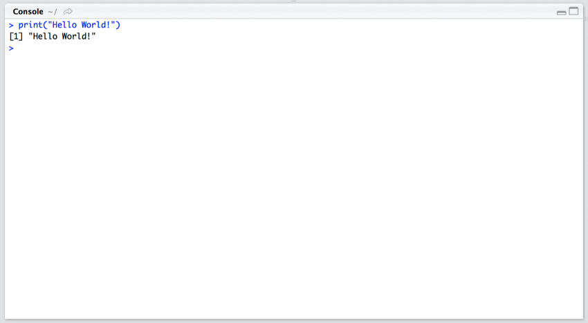
"Hello World"
Congrats! You have just run your first R command.
R comes loaded with help and code examples. You can also find a lot of help on the web. One good source of help is
Stackoverflow
, particulary in the
R section. There is also an interesting blog post on Stackoverflow on the
growth of R.
We are now going to look at how to get some help with commands.
You see a line of code that says
protein_conc <- c(0.0, 0.2, 0.4, 0.6, 0.8, 1.0)
and you can't rtemember what the <- or the c mean.
- In the Console pane (bottom left) type
help("<-") and press return.
The bottom right pane (Files, Plots, Packages, Help and Viewer pane) should now look like the following:
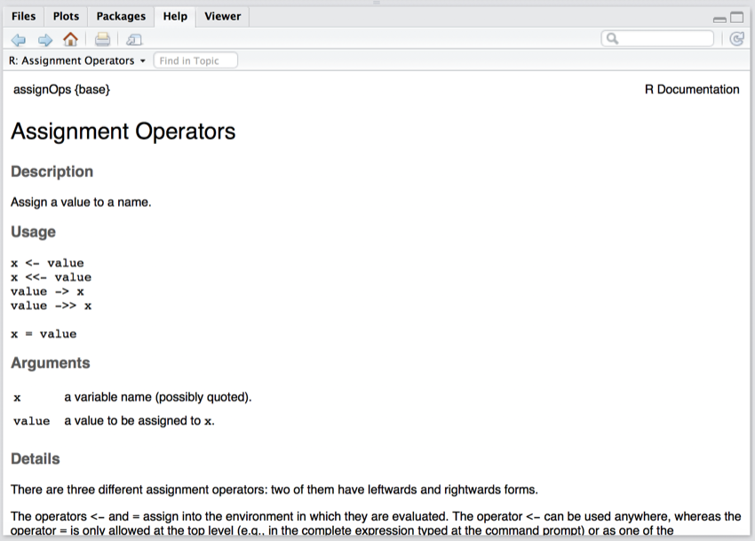
Help information on <-
- In the Console pane (bottom left) type
help("c") and press return.
You should now be viewing some help in the Help pane on c and how it is used.
- Repeat the above for sum, mean, sd and log.
If you type in a command and get it wrong, don't panic, as you can recall and edit the old command by pressing the up-arrow key on the keyboard.
Sometimes you can't remember how to use a command. To get examples just type: example(\"sum\").
- In the Console pane (bottom left) type
example("sum") and press return.
You should now have some examples of how to use the 'sum' command shown in the Console pane.
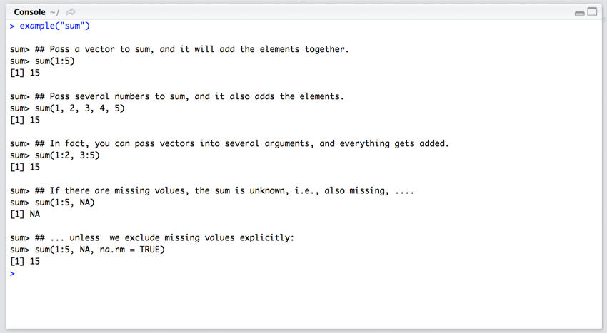
How to use 'sum'
In this section, we are going to write your first R script.
Earlier you opened a new tab called 'Untitle1' in the 'Script and Data' pane. We are now going to add the R script code to it.
- In the new tab copy and paste the following:
       protein_conc <- c(0.0, 0.2, 0.4, 0.6, 0.8, 1.0)
       protein_abs <- c(0.0, 0.31, 0.59, 0.82, 1.21, 1.48)
       standard_data <- data.frame(protein_conc,protein_abs)
       unknowns <- c(0.77,0.14,0.76,0.16,0.42,0.43)
       plot(protein_conc, protein_abs, xlab="Protein Concentration (mg/ml)", ylab="Absorbance (595 nm)", main="Plot of Absorbance (595 nm) against Protein Concentration (mg/ml)")
       fit <- lm(protein_abs ~ protein_conc, data=standard_data)
       abline(fit)
       theAns <- predict(lm(protein_conc ~ protein_abs, data=standard_data), newdata=data.frame(protein_abs=unknowns))
       print(theAns)
The pane should now look like this:
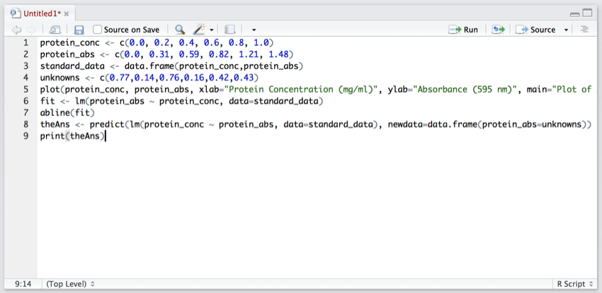
Your first script
You should recognise the script from the lecture on R - it is the protein standard curve script.
We are now going to step through the script and see what each line does. But first, we will Save it.
- Click on the File menu and select Save. Save the file to your script folder.
Now, to run the script.
- Click at the start of the first line of the script - this will return the cursor to the start of the script, so we run from the beginning.
- Note that the 'Environment' (top right) and 'Plots' panes are empty.
- Click on the 'Run' icon (see image below).
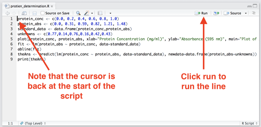
Make sure the cursor is back at the first line of the script, and then click 'Run'
You have just run the first line of code of the script and the RStudio window will have changed and should look similar to the image below.
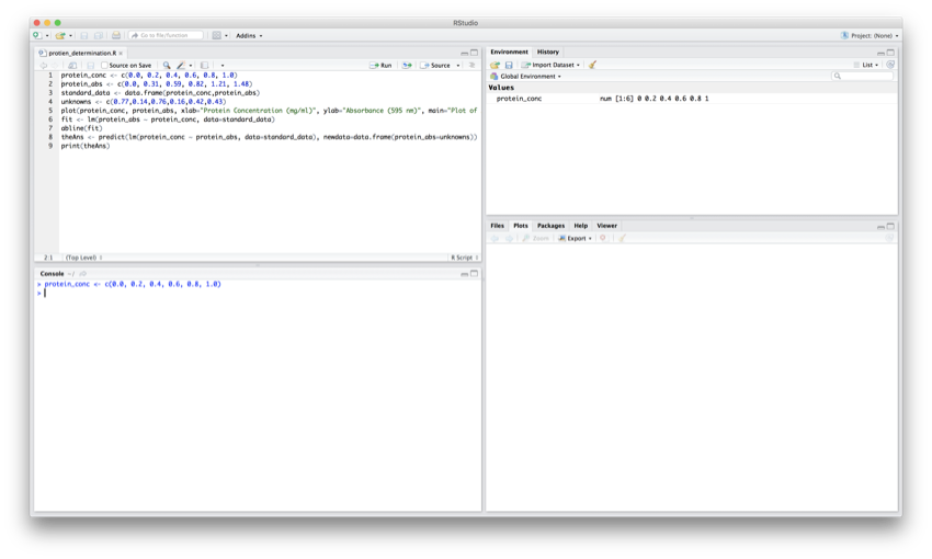
After the first line.
Things to note:
- The cursor has moved down to line 2 of the code
- The vector 'protein_conc' has been created and can be seen in the 'Environment' pane
- The line of code executed has been echoed in the 'Console' pane
- There has been no change to the 'Plots' pane
- Click 'Run' to process line 2 of the code.
You have now created the 'protein_abs' vector, and it should be displayed in the 'Environment' pane
- Click 'Run' to process line 3 of the code.
You have now created the data frame 'standard_data' that contains the 'protein_abs' and 'protein_conc'. Your 'Environment' should look like the image below.
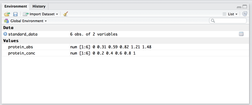
The programming environment after 3 lines of code
We will now review the data in the data frame 'standard_data'.
- In the 'Environment' pane click on the small blue circle with and arrow to the left of 'standard_data'.
You should now be viewing the data in the data frame.
- In the 'Environment' pane click on the grid to the right of 'standard_data'.
This is the equivalent of running 'View(standard_data)' in the 'Console' and 'View(standard_data)' should have appeared in the console.
Also, the data frame should have opened in the 'Script and Data' pane.
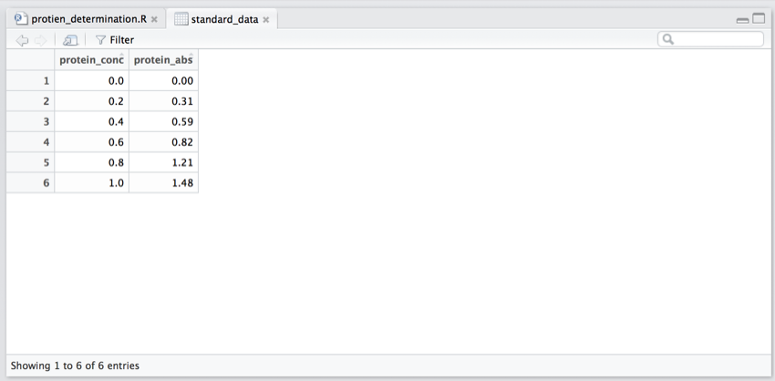
The 'standard_data' data frame
- In the 'Script and Data' pane click on the 'x' on the 'standard_data' to close the tab and return to the script.
- Click 'Run' to process line 4 of the code and create the 'unknowns' vector.
- Click 'Run' to process line 5 of the code.
Line 5 was a 'biggie' as one line of code has drawn a graph, and the graph can now be seen in the 'Plot' pane (bottom right).
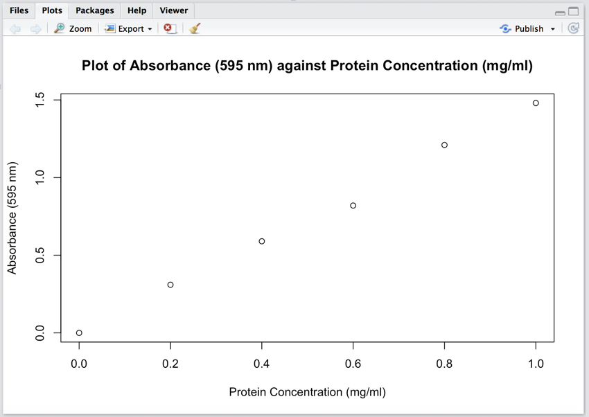
One line of code, line 5, plotted the graph
Let's have a look at the code for the graph. The line was:
plot(protein_conc, protein_abs, xlab="Protein Concentration (µg/µl)", ylab="Absorbance (620 nm)", main="Plot of Absorbance (620 nm) against Protein Concentration (µg/µl)")
The vectors 'protein_conc' and 'protein_abs' contain the data to be plotted. 'ylab' and 'xlab' are the labels for the y and x axes, respectively. And 'main' gives the graph a title.
Next, we are going to put a line of best fit on the graph, but first, we need to build a model of the line, and this is what line 6 does.
- Click 'Run' to process line 6 of the code.
The line
fit <- lm(protein_abs ~ protein_conc, data=standard_data)
is creating the model and storing it in the variable 'fit'. We have passed 'lm' (linear model) the date frame for the plot (standard_data) and data to use to determine the line of best fit. The data to determine the line of best fit is given y ~ x, hence we tell the model which column in data frame 'standard_data' is the x column, i.e. 'protein_conc', and the y column is 'protein_abs'. This means the equation y = mx + c, and the model calculates m and c.
We will now add the line to the graph.
- Click 'Run' to process line 7 of the code.
Your graph should now look like the image below.
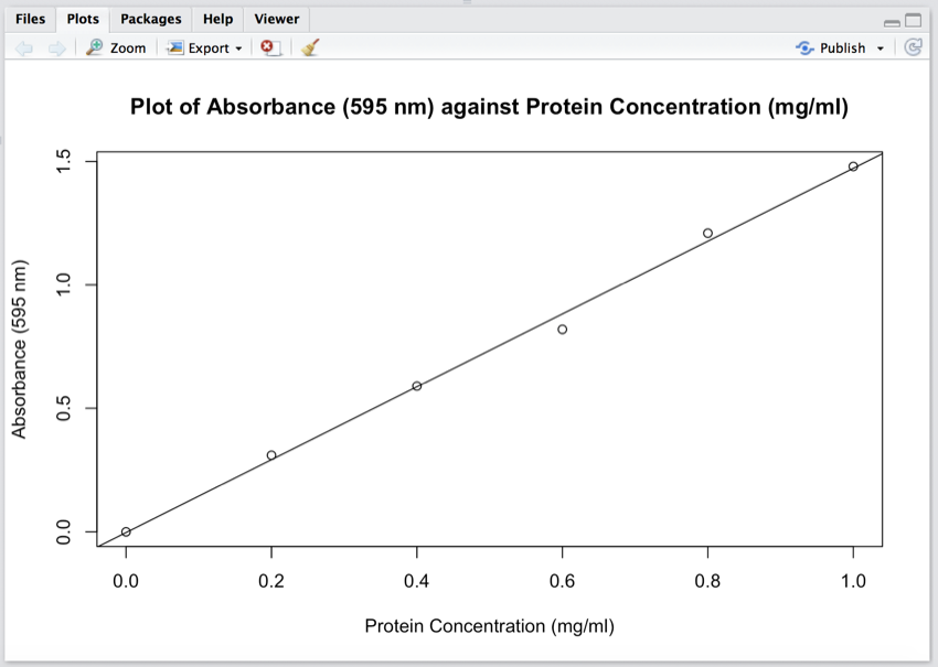
Protein standard curve with the line of best fit.
The next line in the script, line 8, is a bit of an odd line:
theAns <- predict(lm(protein_conc ~ protein_abs, data=standard_data), newdata=data.frame(protein_abs=unknowns))
What this line is doing is producing a new model of the data so we can determine the unknowns. The
lm(protein_conc ~ protein_abs, data=standard_data)
part of the line is the new model. You may have noticed that we have reversed the x and the y in the lm call from what we did in line 6.
The reason we have reversed them is because in the original model in line 6 we designed it to predict values of y (absorbance) for given values of x (protein concentration) i.e. the measured (dependent) againt the concentration (independent). However, now we need to predict values of protein concentration for given absorbances, hence the reverse.
The 'predict' command takes the new model and then uses it to process the new data in a data frame that is created in the call with the with the code:
newdata=data.frame(protein_abs=unknowns)
- Click 'Run' to process line 8 of the code.
You have now created a new vector, 'theAns' containing the predicted protein concentrations for the unknowns.
- Finally, Click 'Run' to process line 9 of the code.
The Console should now contain a data dump of the 'theAns' vector.
Congratulations! You have run your first script and determined the protein concentration of six unknowns.
You are now going to edit the script to use the following new data.
You have run a new protein determination assay in the lab. The absorbances in this new assay were measured at 620 nm.
- Known protein concentrations (µg/µl): 0.0, 0.1, 0.2, 0.3, 0.4, 0.5
- Known protein absorbances (A620): 0.0, 0.22, 0.45, 0.68, 0.85, 1.10
- Unknown protein absorbances (A620): 0.15, 0.24 ,0.76, 0.36
What is the concentration of the unknowns?
Add one line of code to the end of the script to create a data frame called theResults which contains your unknowns and your answers.
In the lecture I introduced two possible systems that would allow you to learn R.
- Data camp free course - WARNING: You have to give an email address and then they 'spam' you with information about paid courses
- Swirl - this is free and runs in RStudio
Of the two above, I would recommend
Swirl. It may not be as 'pretty' as the Datacamp training material, but it gets the job done, it is free, and you don't get spammed.
To get
Swirl running in RStudio you do need to install a 'package' and set the system up, but it is fairly straight forward and it is explained very nicely on their
Swirl - student start page. On their page, start at Step 3 as you already have RStudio installed.
OK, there is a lot more to R and RStudio than we have covered here, but I hope that the above has given you a start and you can see and recognise the full power and potential of R.
Enjoy!